Handbag Brand detection

Summary

In order to identify the brand of handbags, a deep neural network was built to recognize images from scratch with a precision of 97% and recall of 96% while explaining the techniques used throughout the process.

Problem Statement

Machine learning are one of essential data science tools for businesses to understand their content and how their users/consumer interact with it. These efforts have mainly focused on Natural Language Processing (NLP) where we have created tools that can automatically detect topics, entities (e.g., people, organizations, products), and keywords in an article published by any of their products. This information serves as useful building blocks for other tools to improve both the user and editorial experience.

Apart from textual content, most online retail stores and e-commerce platforms include vivid videos and images. These graphical media provide exciting frontiers where we can utilize and Machine Learning to enhance reach to the right users. Building data products which are able to recognize uique and vivid images, we are able to further understand the sentiments, insights and preferences of users on e-commerce platforms or within a location. Companies will be able to anticipate incoming demand of potentially profitable items.

Why handbags?

The undeniable competition between different e-commerce giants producing in-house data products such as Asos mobile application and Zalando shows that there is immense commercial value in data product. After considering different components of a data product by online retail stores such as recommender system and image recognition tech, this projects will focus on creating a prototype handbag brand classifier. Luxury handbags will be the focus of this project as they are highly sensationalised objects from the fashion domain. Moreover, from a computer vision perspective, handbags are rather complicated objects within an image. Many luxury brands have design distinct features which differentiates them visually. These features range from the more obvious (e.g., patterns, logos) to the less visible (e.g., textures, pockets, latches, straps). Of course, any fashion IT girl can give an accurate prediction of the handbag’s brand without physically inspecting the handbag. How are we suppose to identify which brand is the hottest each season without a classifier on social media?

Introduction

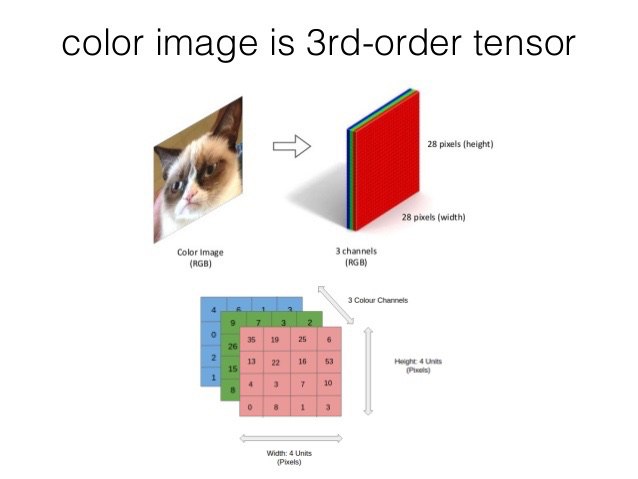
Before we go into complex concepts such as machine learning and neural network, we must understand how the computer views images. Computers extract images based on the pixels they present. In coloured images as RGB values ( list of numbers which represent the combination of red, green and blue from a nubmer range of 0 to 255). Computers could then extract the RGB value of each pixel and put the result in an array for interpretation.

In this project, we will class each brand to the images in the data set. Thus, a new image is added into the computer, it interprets a new image, it will convert the image to an array by using the same technique, which then compares the patterns of numbers against the already-known objects. The computer then allots confidence scores for each class. The class with the highest confidence score is usually the predicted one. This is done by machine learning.

Machine learning: Algorithms that can make predictions through pattern recognition

Why is this a machine learning project?

There are three main factors that differentiates a machine learning project and a deep learning (DL) algorithm. The first is the size of the data points. Most machine learning (ML) algorithm are in the range of 100-10000 data points while deep learning algorithm require at least a million data points. The second factor is the amount of supervision of the neural network requires. ML algorithm requires much more supervision in terms of selecting optimizers, regularisation and the quality of the data set. On the other hand, DL algorithm develop the neural networks as more information inserted into it. Lastly, DL algorithm requires more computing power than ML algorithm.

How do machine learning algorithm process their data?

They use neural networks

Neural Networks: A Neural Network consists of an interconnected group of nodes called neurons. The input feature variables from the data are passed to these neurons as a multi-variable linear combination, where the values multiplied by each feature variable are known as weights. A non-linearity is then applied to this linear combination which gives the neural network the ability to model complex non-linear relationships.

Why is Convolutional Neural Network applicable for image?

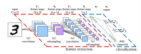
The convolutional neural networks make a conscious tradeoff: if a network is designed for specifically handling the images, some generalizability has to be sacrificed for a much more feasible solution.

If you consider any image, proximity has a strong relation with similarity in it and convolutional neural networks specifically take advantage of this fact. This implies, in a given image, two pixels that are nearer to each other are more likely to be related than the two pixels that are apart from each other. Nevertheless, in a usual neural network, every pixel is linked to every single neuron. The added computational load makes the network less accurate in this case.

By killing a lot of these less significant connections, convolution solves this problem. In technical terms, convolutional neural networks make the image processing computationally manageable through filtering the connections by proximity. In a given layer, rather than linking every input to every neuron, convolutional neural networks restrict the connections intentionally so that any one neuron accepts the inputs only from a small subsection of the layer before it(say like 55 or 33 pixels). Hence, each neuron is responsible for processing only a certain portion of an image.(Incidentally, this is almost how the individual cortical neurons function in your brain. Each neuron responds to only a small portion of your complete visual field).

Project Workflow

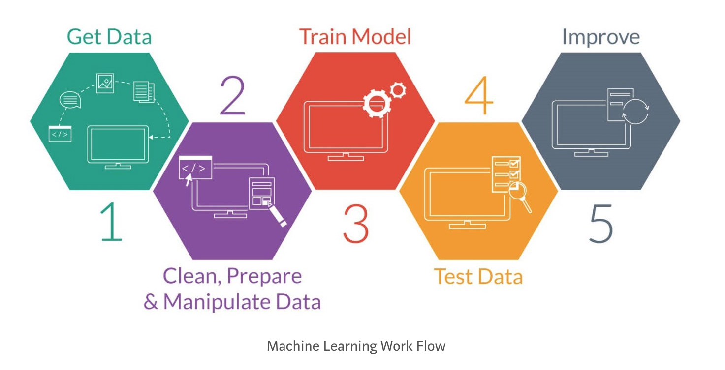
This project have 5 main stages. We scrap images from Google Images to “Get Data” in Stage 1. Stage 2 requires us to manual review the images scrap, conduct image augmentation on the training data set and label the images. Stage 3 is where we build the model using Keras with a TensorFlow backend. This step is done through applying VGGnet-inspired architecture without a pre-trained layer. Stage 4 allows us to test the accuracy of our model with a new set of images.

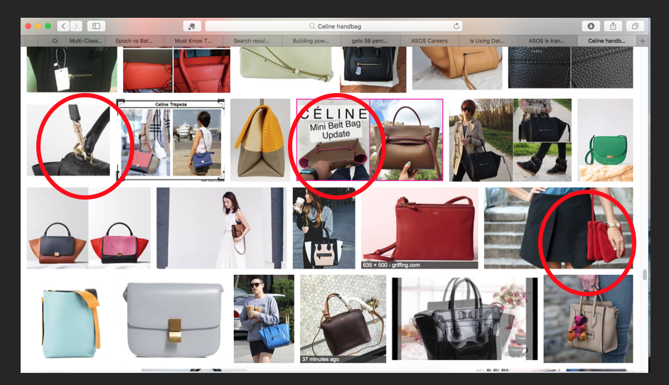
Dataset

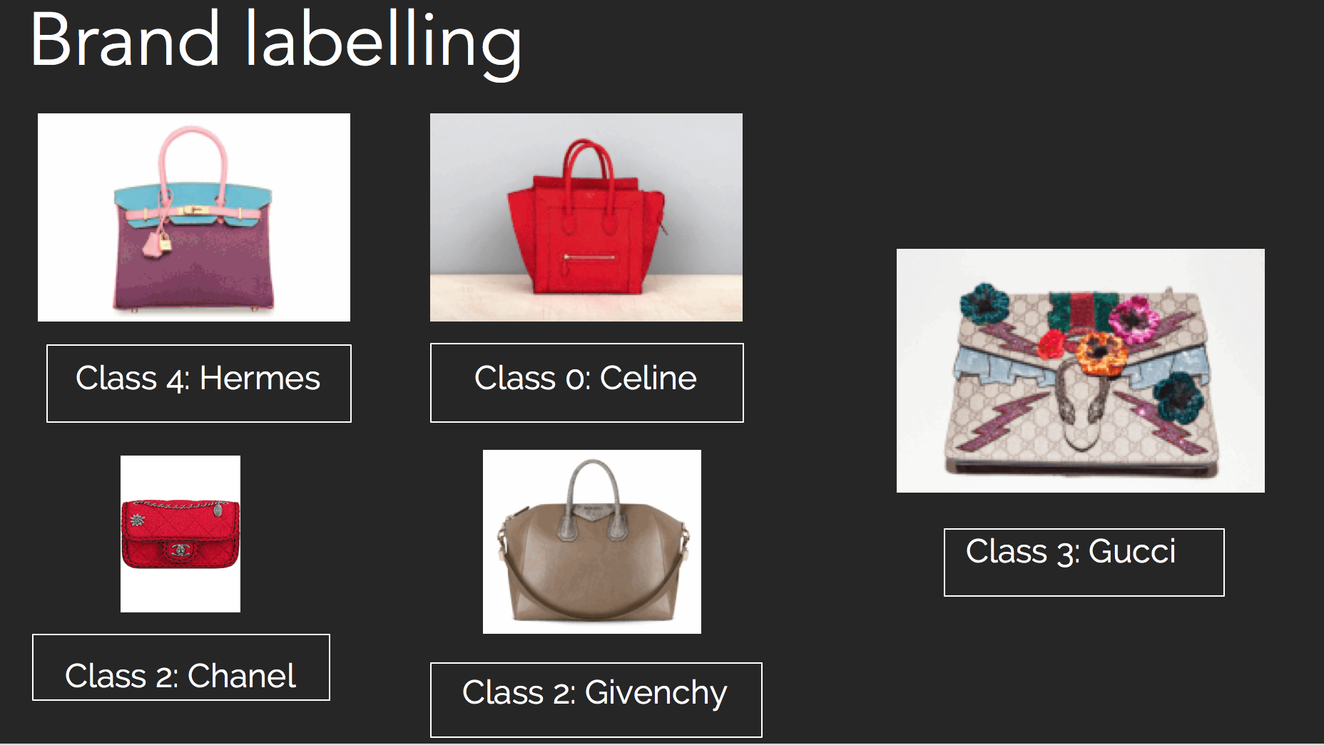
The dataset used in this classifier was collected from Google Images using personalised google search. With Selenium, BeautifulSoup and urllib, the images are collected locally and reviewed manually before being included into the finalised dataset. The data contains selfies, ‘outfit of the day’ and amateur images. Each image in the dataset can only include one image as the prototype does not include object localisation. In total, we collected an evenly-distributed dataset of 7,500 images across 5 brands:

Brands

• Celine
• Chanel
• Givenchy
• Gucci
• Hermes

Stage 1:Scraping Images

'''The handbag brands are stored in a csv files'''
bags=pd.read_csv("./bag.csv")
handbagnames=bags.values.T.tolist()[0]
typeofbags=bags.values.T.tolist()[0]
url=[]

for handbag in handbagnames:
    url += ["https://www.google.com/search?q=handbag%20purse%20"+handbag+"&source=lnms&tbm=isch"]
    
driver = webdriver.Chrome(executable_path="/Users/hayatibintehamzah/Documents/GitHub/DSIstuff/Capstone/chromedriver")

driver.get(url[0])
WebDriverWait(driver, timeout=100)
time.sleep(20)
page_source = driver.page_source
page_source = page_source[page_source.find("Search Results"):]
soup = BeautifulSoup(page_source, "html.parser")
images = [a.get('src') for a in soup.find_all("img")]
skipped_imgs=0
item = 0
for img in images:
'''    if not os.path.exists("%s" %(img)):'''    
print("adding %s to folder" %(img))
    try:
        with urllib.request.urlopen(img) as response, open("handbag_crossbody_%s_img_%s.jpg" %(handbagnames[4], item), 'wb') as out_file:
            print(img)
            shutil.copyfileobj(response, out_file)
    except:
        pass
    item +=1

Stage 2:Pre-processing

Setup

import os,cv2
import itertools
import numpy as np
import matplotlib.pyplot as plt
from sklearn.metrics import classification_report,confusion_matrix

import keras
from keras import backend as K
from keras import optimizers,applications
from keras.engine.topology import Input
from keras.utils import to_categorical, np_utils
from keras.models import load_model
from keras.models import Sequential, load_model
from keras.preprocessing.image import ImageDataGenerator
from keras.layers import Conv2D, MaxPooling2D
from keras.layers import Activation, Dropout, Flatten, Dense

Manual clean-up of dataset

The data used here was collected from Google Image using Selenium and BeautifulSoup. All the images were reviewed manually before being added to the dataset. The data contains selfies and other amateur images, white background studio style images, professional fashion and runway images. An image was allowed to contain more than one handbag but since we did not include any object detection we only included multiple handbags if they were the same brand. Images with “Outfit of the Day’ shots where the hangbag cannot be seen clearly, the image is removed. Amateur photos which did not hightlight the key features of handbag was removed too.

Image Augmentation & Splitting dataset

A training data directory and validation data directory containing one subdirectory per image class, filled with .jpg images:

data/
    train/
        Celine/
            handbag_celine_img_0.jpg
            handbag_celine_img_1.jpg
            ...
        Chanel/
            handbag_chanel_img_0.jpg
            handbag_chanel_img_1.jpg
            ...
        Gucci/
            handbag_gucci_img_0.jpg
            handbag_gucci_img_1.jpg
            ...
       Givenchy/
            handbag_givenchy_img_0.jpg
            handbag_givenchy_img_1.jpg
            ...
       Hermes/
            handbag_hermes_img_0.jpg
            handbag_hermes_img_1.jpg
            ...
    validation/
        Celine/
            handbag_celine_img_0.jpg
            handbag_celine_img_1.jpg
            ...
        Chanel/
            handbag_chanel_img_0.jpg
            handbag_chanel_img_1.jpg
            ...
        Gucci/
            handbag_gucci_img_0.jpg
            handbag_gucci_img_1.jpg
            ...
       Givenchy/
            handbag_givenchy_img_0.jpg
            handbag_givenchy_img_1.jpg
            ...
       Hermes/
            handbag_hermes_img_0.jpg
            handbag_hermes_img_1.jpg
            ...

In order to make the most of our few training examples, we will “augment” them via a number of random transformations, so that our model would never see twice the exact same picture. This helps prevent overfitting and helps the model generalize better.

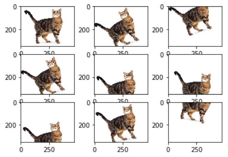
Image augmentation artificially creates training images through different ways of processing or combination of multiple processing, such as random rotation, shifts, shear and flips, etc. An augmented image generator can be easily created using ImageDataGenerator API in Keras. ImageDataGenerator generates batches of image data with real-time data augmentation. The most basic codes to create and configure ImageDataGenerator and train deep neural network with augmented images are as follows.

'''this is the augmentation configuration we will use for training'''
train_datagen = ImageDataGenerator(
    rescale=1. / 255,
    shear_range=0.2,
    zoom_range=0.2,
    horizontal_flip=True)
'''this is the augmentation configuration we will use for testing: only rescaling'''
test_datagen = ImageDataGenerator(rescale=1. / 255)
train_generator = train_datagen.flow_from_directory(
    train_data_dir,
    target_size=(img_width, img_height),
    batch_size=batch_size,
    class_mode='categorical')
validation_generator = test_datagen.flow_from_directory(
    validation_data_dir,
    target_size=(img_width, img_height),
    batch_size=batch_size,
    class_mode='categorical')

Labelling of brands

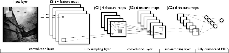
Stage 3: Building a Convolutional Neural Network

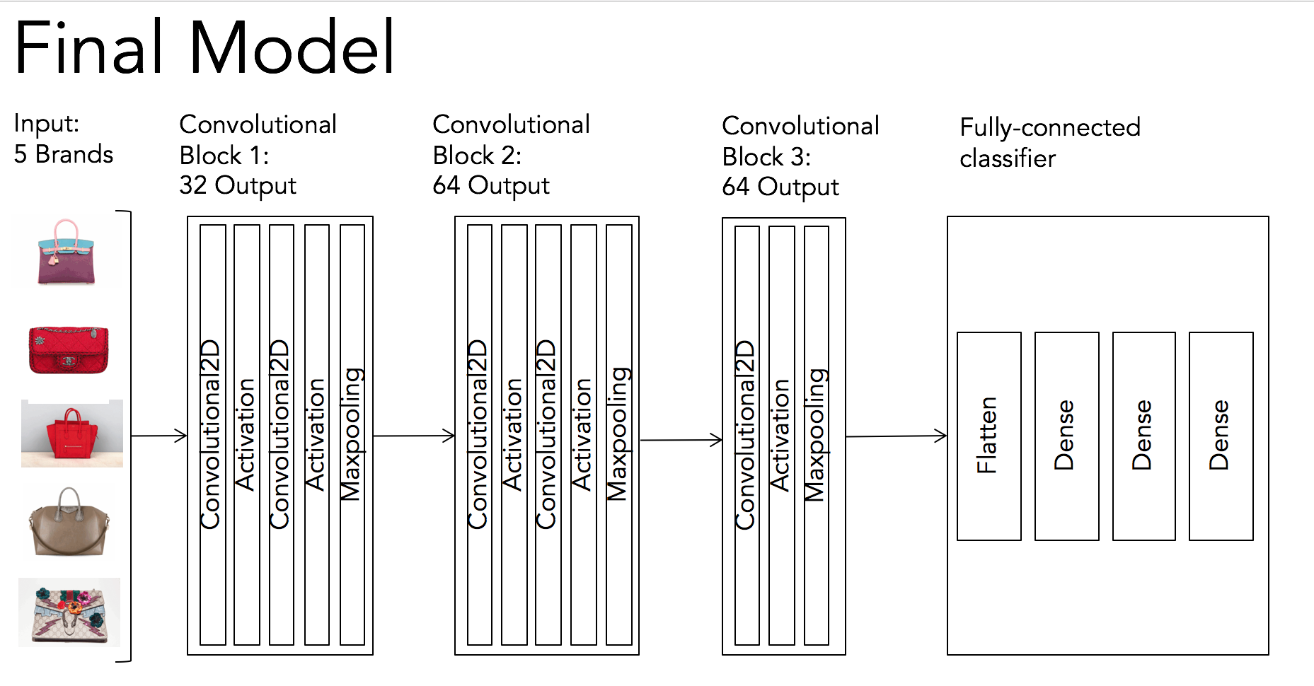
With the completion of the pre-processing and spliting of our dataset, we can start building our neural network. The most successful neural network for this project has 3 stacks of doubled-layered convolutional layers with 2x2 maxpooling layer at the end of each stack. These are the basic neural network layers used in this project:

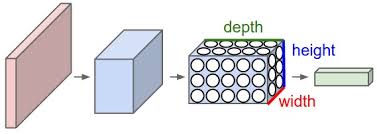
Convolutional: This layer will compute the output of neurons that are connected to local regions in the input, each computing a dot product between their weights and a small region they are connected to in the input volume. This may result in volume such as [32x32x64] if we decided to use 64 filters

Activation: The layer which consist of the activation function which determines what output a node will generate base upon its input

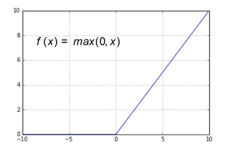
We’ve selected the ‘Relu’ and ‘Softmax’ activation functions. ‘RELU’ function will apply an elementwise activation function, such as the max(0,X) thresholding at zero. This leaves the size of the volume unchanged ([32x32x12]).

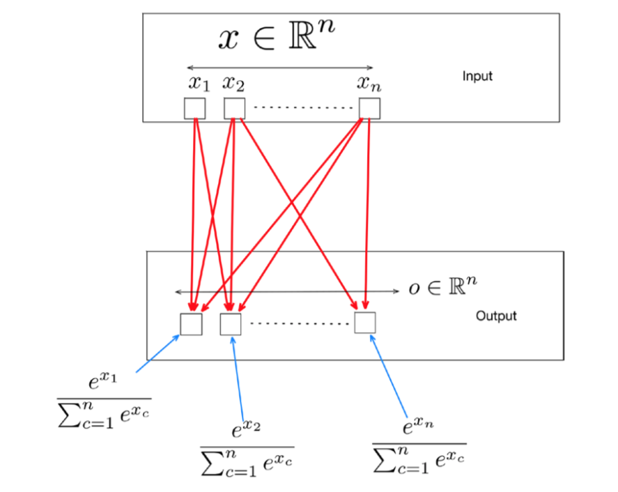
‘Softmax’ function is an extension of the sigmoid function to the multiclass case in conjunction with the Cross Entrophy loss function(formula in the diagram above. The Softmax layer normalizes outputs of the previous layer so that they sum up to one. Typically, the units of the previous layer model an un-normalized score of how likely the input is to belong to a particular class. The softmax layer normalized this so that the output represents the probability for every class.

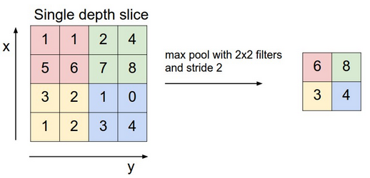
Max-pooling: Layer which takes the largest value from one patch of an image, places it in a new matrix next to the max values from other patches, and discards the rest of the information contained in the activation maps from the activation layer.

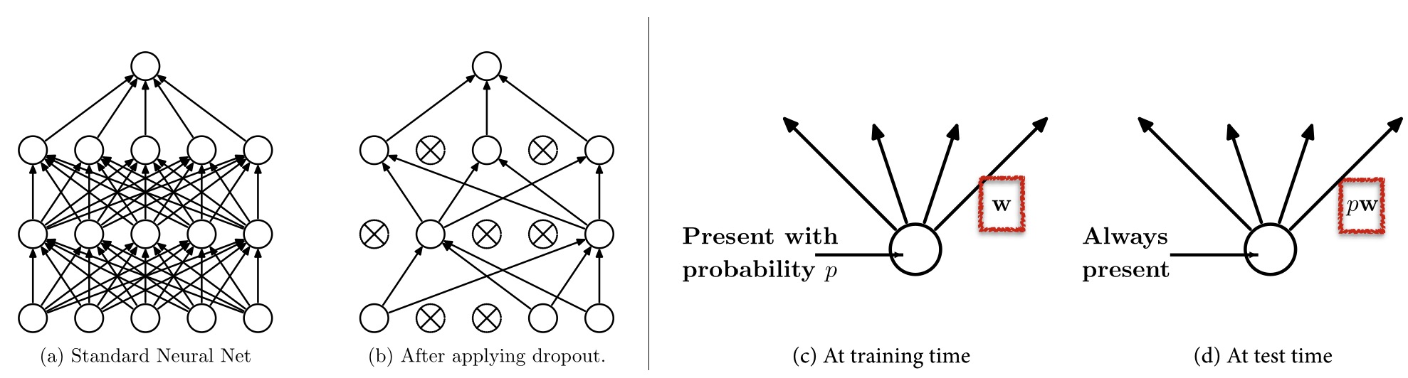
Dropout: The layer where it regularizes the parameters within the network. During training, dropout is implemented by only keeping a neuron active with some probability p (a hyper-parameter), or setting it to zero otherwise.

Model Code:

num_classes = 5
model = Sequential()
model.add(Conv2D(32, (3, 3), input_shape=input_shape))
model.add(Activation('relu'))
model.add(Conv2D(32, 3, 3))
model.add(Activation('relu'))
model.add(MaxPooling2D(pool_size=(2, 2)))

model.add(Conv2D(64, (3, 3)))
model.add(Activation('relu'))
model.add(Conv2D(64, 3, 3))
model.add(Activation('relu'))
model.add(MaxPooling2D(pool_size=(2, 2)))

model.add(Conv2D(64, (3, 3)))
model.add(Activation('relu'))
model.add(MaxPooling2D(pool_size=(2, 2)))

model.add(Flatten())
model.add(Dense(128))
model.add(Activation('relu'))
model.add(Dropout(0.5))
model.add(Dense(num_classes))
model.add(Activation('softmax'))

model.compile(loss='categorical_crossentropy',
              optimizer='Adam',
              metrics=['accuracy'])

Stage 4: Testing the model

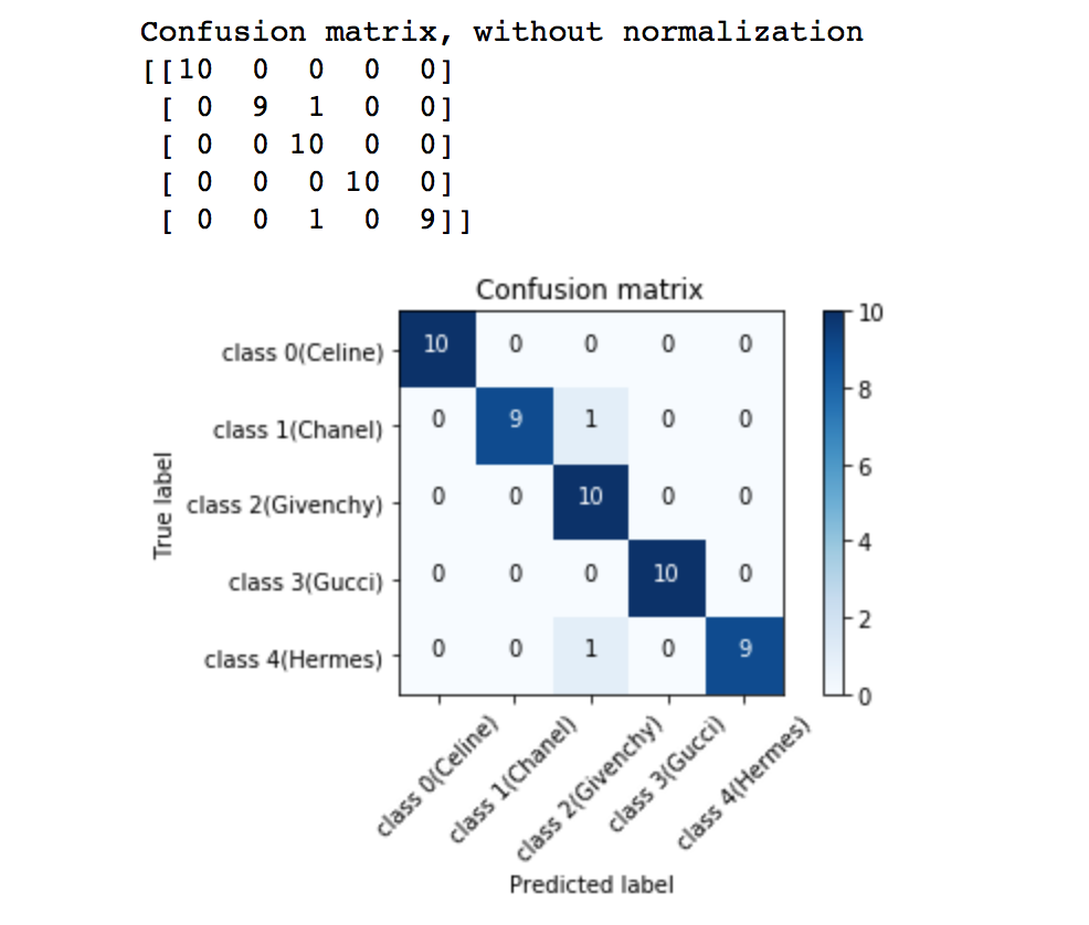
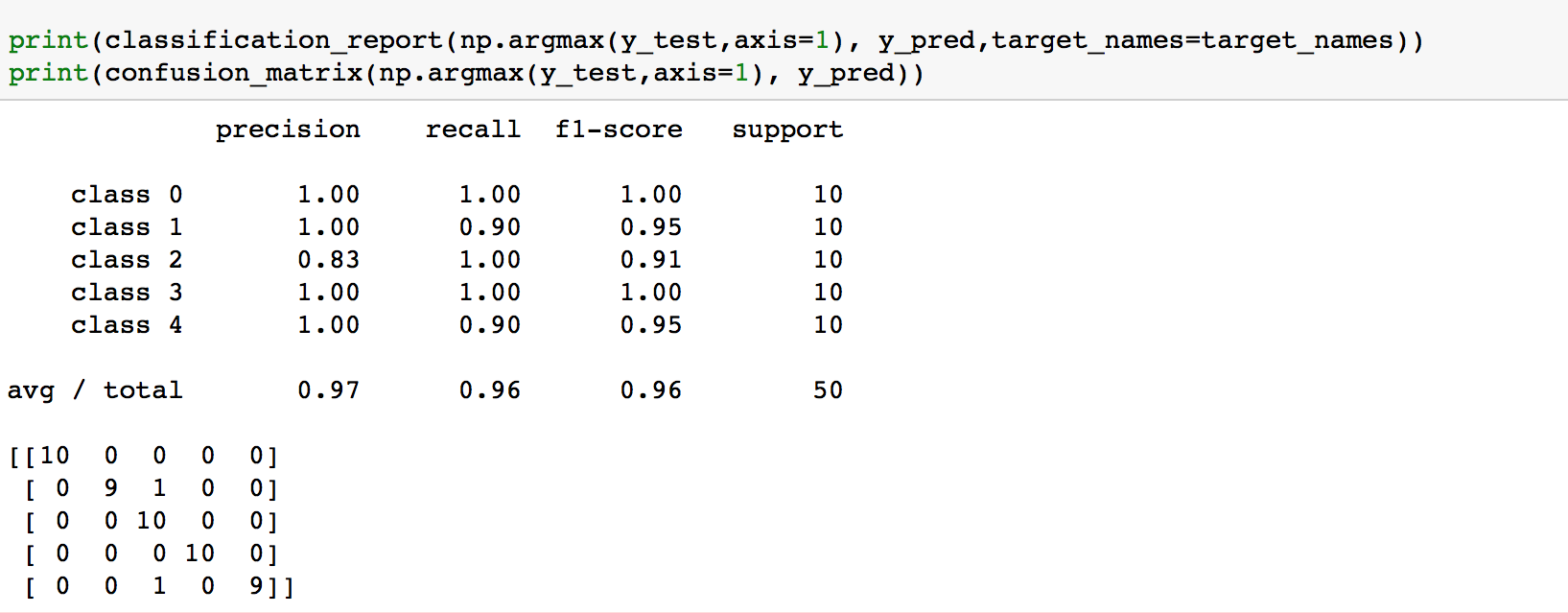
Once we attain our trained neural network, we can test it out on a brand-new dataset! The model manage to interpret 50 handbag images and got an accuracy of 96% (48/50).

Conclusion

There are 3 main things about this project. Quality of data set. Image augmentation and

Future project

Expand dataset

In order to have a versatile dataset, we need to include more brands into the data set and train it. With more data, we hope to include necessary measures such as using transfer learning.

Web app

A Web application where user can insert their images and get the brands of their handbags would make the model much more accessible.